Cross validation은 어떨때 유의미하게 사용될 수 있는가?
1. 데이터의 크기가 매우 커서 나눠지는 데이터의 분포를 담보할 수 없을 때
2. 모델의 복잡도가 매우 높아서 데이터의 특성에 따라 결과가 바뀔 때
3. 대부분의 경우
1. 데이터 전처리 및 EDA
(1) 데이터로드 및 확인

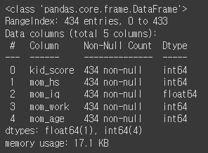
데이터를 먼저 불러와서 확인해줍니다.
5열 434행짜리 크지 않은 데이터 입니다.
(2) 라이브러리 import
import numpy as np
import pandas as pd

import matplotlib as mpl
import matplotlib.pyplot as plt

import patsy
from patsy import dmatrices
import statsmodels
import statsmodels.api as sm #Application Programming Interface
import statsmodels.formula.api as smf
from statsmodels.iolib.summary2 import summary_col

from sklearn.preprocessing import StandardScaler

from sklearn.model_selection import train_test_split, cross_val_score, KFold
from sklearn.metrics import r2_score, explained_variance_score
from sklearn.metrics import mean_squared_error, mean_absolute_error

from sklearn.dummy import DummyRegressor
from sklearn.linear_model import LinearRegression, RidgeCV, LassoCV, ElasticNetCV

import warnings
warnings.filterwarnings('ignore')
필요한 라이브러리 먼저 import!
(3) 데이터 형태 확인
info로 데이터 형태도 확인!
# Target이 NaN인 데이터 탐색
kidiq[kidiq['kid_score'].isna()].head()
info로 널값이 없는것을 확인했지만, 확실하게 더블체크해주기
kidiq.describe()
데이터를 상세하게 뜯어봤을때, 옛날 데이터라 그런지 엄마들의 나이가 평균 22세로 꽤나 낮네요
mom_hs는 엄마의 고등학교 졸업 여부를 나타내는데 약 80%정도가 졸업을 한것으로 보입니다.
# 추가 컬럼 생성
kidiq['mom_iq_c'] = kidiq['mom_iq'] - kidiq['mom_iq'].mean()
kidiq['mom_age_c'] = kidiq['mom_age'] - kidiq['mom_age'].mean()
kidiq
엄마의 아이큐와 나이가 평균보다 얼마나 떨어져있는지 확인하기 위해서 추가컬럼을 생성해줬습니다.
(4) 데이터 분포 확인
kidiq.hist(figsize=(21,8))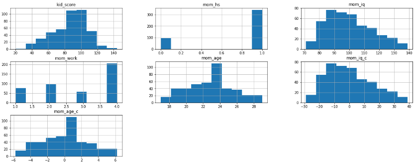
데이터는 항상 눈으로 보는게 중요하니 히스토그램, 박스플롯 등 직접 눈으로 확인하고 넘어가자
위의 describe로 확인했을때 아이들의 iq가 평균 86이지만 그래프로 봤을때엔 100구간이 제일 많은것을 확인할 수 있다
2. EDA 결과 시각화
(1) EDA 결과
# Fit regression model using centered version of mom_iq
# OLS: Ordinary Least Squares)
# 에러(잔차)의 제곱합 (RSS: Residual Sum of Squares)를 최소화하는 가중치 벡터를 구하는 방법
fit1 = smf.ols('kid_score ~ 1 + mom_hs + mom_iq_c + mom_age_c', data=kidiq).fit()

# 1+ ? + ? + ?
# Inspect results
print(fit1.summary())
ols모델은 처음 써보는데, R기반의 모델이라 코드도 R처럼 사용을 한다.
y = kidiq['kid_score']
X = kidiq[['mom_hs', 'mom_iq_c', 'mom_age_c']]
X = sm.add_constant(X)

model1 = sm.OLS(y,X)

res1 = model1.fit()

print(res1.summary())
파이썬코드로 변경을 하려면 이렇게 사용하면 된다!
동일한 결과값을 출력한다
features = res1.params.index
coefs = [round(val, 4) for val in res1.params.values]

dict(zip(features, coefs))
>> {'const': 82.3602, 'mom_hs': 5.6472, 'mom_iq_c': 0.5625, 'mom_age_c': 0.2248}
print("In-samle R-squared: %.3f" % round(res1.rsquared, 3))>> In-sample R-squared: 0.215
print("In-sample RMSE: %.3f" % round(np.mean((y - res1.fittedvalues)**2)**0.5, 3))>> In-sample RMSE: 18.063
주요 수치들을 확인해보자 R-square값은 높을수록, RMSE값은 낮을수록 좋은데 R-square값이 썩 좋지는 않다.
(2) 시각화
def abline(intercept, slope, **params):
    axes = plt.gca()
    x_vals = np.array(axes.get_xlim())
    y_vals = intercept + slope * x_vals
    plt.plot(x_vals, y_vals, '-', **params)
fig, ax = plt.subplots(figsize=(10, 6))
colors = {1:'red', 0:'blue'}
b_hat = fit1.params
ax.scatter(kidiq.mom_iq_c, kidiq.kid_score, color=kidiq.mom_hs.map(colors))
sm.graphics.abline_plot(intercept=b_hat['Intercept'], slope=b_hat['mom_iq_c'], color='blue', label='No HS', ax=ax)
sm.graphics.abline_plot(intercept=b_hat['Intercept']+b_hat['mom_hs'], slope=b_hat['mom_iq_c'], color='red', label='HS', ax=ax)
ax.set_ylabel('Kid Score', fontsize=14)
ax.set_xlabel('Mom IQ (centered)', fontsize=14)
ax.legend(fontsize=11)
ax.set_title('Linear Regression\n$R^2= %.2f$' % fit1.rsquared_adj, fontsize=18)
fig.tight_layout();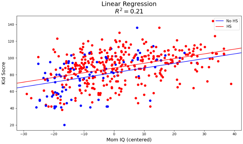
엄마의 아이큐가 평균에 얼마나 멀어졌는지에 따라 아이들의 아이큐 분포가 어떻게 생겼는지 확인해보자.
고등학교 졸업 여부가 가장큰 영향을 끼치는 피쳐로, 시각화에 사용하였습니다.
3. Cross validation
(1) K-fold cross validation using statsmodels and scikit-learn
len(y), round(len(y)*(4/5))>> (434, 347)
먼저 fold를 5개로 나누기 위해서 데이터의 갯수를 확인해줬습니다.
y = kidiq['kid_score']

X = kidiq[['mom_hs', 'mom_iq_c']]
X = sm.add_constant(X)

X[:5]
X값과 y값도 넣어줍니다.

(2) R-squared
kfold = KFold(n_splits=5, shuffle=True, random_state=123)

scores = []
for k, (train, test) in enumerate(kfold.split(X, y)):
    res1 = sm.OLS(y[train], X.loc[train,:]).fit()
    preds = res1.predict(X.loc[test,:])
    score = r2_score(y[test], preds)
    scores.append(score)
    print('Fold: {:2d}, Training size: {}, Out-of-sample R-squared: {:.3f}'.format(k+1, len(y[train]), score))

print('\nCV R-squared: {:.3f} (+/- {:.3f})'.format(np.mean(scores), np.std(scores)))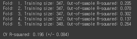
R-squared 값이 0.196으로 낮은 수치가 나왔습니다.
(3) RMSE
kfold = KFold(n_splits=5, shuffle=True, random_state=123)

scores = []
for k, (train, test) in enumerate(kfold.split(X, y)):
    res1 = sm.OLS(y[train], X.loc[train,:]).fit()
    preds = res1.predict(X.loc[test,:])
    score = mean_squared_error(y[test], preds, squared=False)
    scores.append(score)
    print('Fold: {:2d}, Training size: {}, Out-of-sample RMSE: {:.3f}'.format(k+1, len(y[train]), score))

print('\nCV RMSE: {:.3f} (+/- {:.3f})'.format(np.mean(scores), np.std(scores)))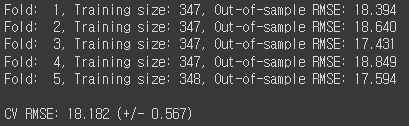
RMSE값은 18.182로 EDA와 비슷한 결과가 나왔습니다.
(4) interaction term
조금더 좋은 값을 내기 위해서 X에 값을 추가해줬습니다.
y = kidiq['kid_score']

kidiq['mom_hs_iq_c'] = kidiq['mom_hs'] * kidiq['mom_iq_c']

X = kidiq[['mom_hs', 'mom_iq_c', 'mom_hs_iq_c']]
X = sm.add_constant(X)

X[-5:]
위에서는 단순히 엄마의 고등학교졸업여부와 iq를 넣었다면 이번엔 졸업여부와 iq의 interaction을 추가해서 넣어주었습니다.
interaction term을 넣은 이유는 한 독립변수의 변화가 "또다른 독립변수의 종속변수 Y에 대한 영향력을 어떻게 변경"하는지를 알아보기 위해서입니다.
kfold = KFold(n_splits=5, shuffle=True, random_state=123)

scores = []
for k, (train, test) in enumerate(kfold.split(X, y)):
    res1 = sm.OLS(y[train], X.loc[train,:]).fit()
    preds = res1.predict(X.loc[test,:])
    score = r2_score(y[test], preds)
    scores.append(score)
    print('Fold: {:2d}, Training size: {}, Out-of-sample R-squared: {:.3f}'.format(k+1, len(y[train]), score))

print('\nCV R-squared: {:.3f} (+/- {:.3f})'.format(np.mean(scores), np.std(scores)))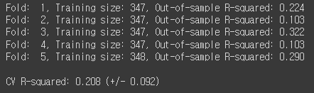
0.196 -> 0.208로 R-squared 값이 증가한것을 확인할 수 있었습니다.
kfold = KFold(n_splits=5, shuffle=True, random_state=123)

scores = []
for k, (train, test) in enumerate(kfold.split(X, y)):
    res1 = sm.OLS(y[train], X.loc[train,:]).fit()
    preds = res1.predict(X.loc[test,:])
    score = mean_squared_error(y[test], preds, squared=False)
    scores.append(score)
    print('Fold: {:2d}, Training size: {}, Out-of-sample RMSE: {:.3f}'.format(k+1, len(y[train]), score))

print('\nCV RMSE: {:.3f} (+/- {:.3f})'.format(np.mean(scores), np.std(scores)))
RMSE 값도 미세하지만 감소한것을 확인할 수 있었습니다.
(5) fold를 10개로 늘린다면?
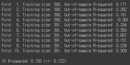

데이터의 양이 적어서 그런지 RMSE값은 감소하였으나, R-squared 값도 같이 감소하였습니다.
많은 양의 데이터가 아니라 10개까지 fold를 나눌 필요는 없어 보입니다.
(6) Kfold cross validation 손코딩
y = kidiq['kid_score'].values
X = kidiq[['mom_hs', 'mom_iq_c']]
X = sm.add_constant(X)
X = X.values
y
손코딩을 하는 이유는 array받은 데이터를 numpy로 사용한다면 모델의 속도가 훨씬 빨라지기 때문입니다.
n_samples = len(y)
indices = np.arange(n_samples)

n_splits = 5
num_val_samples = np.full(n_splits, n_samples // n_splits, dtype=int)
num_val_samples[: n_samples % n_splits] += 1

scores = []
for i in range(n_splits):
    start =  i      * num_val_samples[i]
    stop  = (i + 1) * num_val_samples[i] # data [0:84]
    y_test = y[indices[start:stop]]
    X_test = X[indices[start:stop], :]
    y_train = np.concatenate([ y[indices[:start]] ,
                               y[indices[stop:]] ] , axis=0)
    X_train = np.concatenate([ X[indices[:start], :] ,
                               X[indices[stop:], :] ] , axis=0)

    res1 = sm.OLS(y_train, X_train).fit()
    score = res1.rsquared
    scores.append(score)
    print('Fold: {:2d}, Training size: {}, Out-of-sample R-squared: {:.3f}'.format(i+1, len(y_train), score))

print('\nCV R-squared: {:.3f} (+/- {:.3f})'.format(np.mean(scores), np.std(scores)))
y = kidiq['kid_score'].values
X = kidiq[['mom_hs', 'mom_iq_c']]
X = sm.add_constant(X)
X = X.values

n_samples = len(y)
indices = np.arange(n_samples)

n_splits = 5
num_val_samples = np.full(n_splits, n_samples // n_splits, dtype=int)
num_val_samples[: n_samples % n_splits] += 1

scores = []
for i in range(n_splits):
    start =  i      * num_val_samples[i]
    stop  = (i + 1) * num_val_samples[i]
    y_test = y[indices[start:stop]]
    X_test = X[indices[start:stop], :]
    y_train = np.concatenate([ y[indices[:start]] ,
                               y[indices[stop:]] ] , axis=0)
    X_train = np.concatenate([ X[indices[:start], :] ,
                               X[indices[stop:], :] ] , axis=0)

    res1 = sm.OLS(y_train, X_train).fit()
    preds = res1.predict(X_test)
    score = np.mean((y_test - preds)**2)**0.5
    scores.append(score)
    print('Fold: {:2d}, Training size: {}, RMSE: {:.3f}'.format(i+1, len(y_train), score))

print('\nCV RMSE: {:.3f} (+/- {:.3f})'.format(np.mean(scores), np.std(scores)))
R-squared 값이나 RMSE값이나 기존의 결과와 비슷비슷하게 출력이 됩니다.
아무래도 데이터의 양이 적어서 크게 차이가 나지 않지 않나 생각이 들었습니다.
4. LinearRegression
scikit-learn을 이용해서 추가로 분석을 진행해 보았습니다.
y = kidiq['kid_score']
X = kidiq[['mom_hs', 'mom_iq_c']]
lm1 = LinearRegression().fit(X, y)
lm1
먼저 LinearRegression 모델을 생성해주고
coefs = [round(val, 3) for val in list(np.concatenate((lm1.intercept_, lm1.coef_), axis=None))]
features = list(np.concatenate((np.array('Intercept'), lm1.feature_names_in_), axis=None))

dict(zip(features, coefs))
>> {'Intercept': 82.122, 'mom_hs': 5.95, 'mom_iq_c': 0.564}
회귀계수도 확인해줍니다.
위에 OLS모델을 사용했을때와 흡사한 결과를 출력했습니다.
# The in-sample coefficient of determination: 1 is perfect prediction
print("In-sample R-squared: %.3f" % round(lm1.score(X, y), 3))
>> In-sample R-squared: 0.214
print("In-sample RMSE: %.3f" % round(mean_squared_error(y, lm1.predict(X), squared=False), 3))>> In-sample RMSE: 18.073
R-squared와 RMSE값도 흡사하게 나타났습니다.
kfold = KFold(n_splits=5, shuffle=True, random_state=123)

scores = []
for k, (train, test) in enumerate(kfold.split(X, y)):
    lm1.fit(X.loc[train,:], y[train])
    score = lm1.score(X.loc[test,:], y[test])
    scores.append(score)
    print('Fold: {:2d}, Training size: {}, Out-of-sample R-squared: {:.3f}'.format(k+1, len(y[train]), score))

print('\nCV R-squared: {:.3f} (+/- {:.3f})'.format(np.mean(scores), np.std(scores)))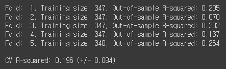
kfold = KFold(n_splits=5, shuffle=True, random_state=123)

scores = []
for k, (train, test) in enumerate(kfold.split(X, y)):
    lm1.fit(X.loc[train,:], y[train])
    preds = lm1.predict(X.loc[test,:])
    score = mean_squared_error(y[test], preds, squared=False)
    scores.append(score)
    print('Fold: {:2d}, Training size: {}, Out-of-sample RMSE: {:.3f}'.format(k+1, len(y[train]), score))

print('\nCV RMSE: {:.3f} (+/- {:.3f})'.format(np.mean(scores), np.std(scores, ddof=1) * 2))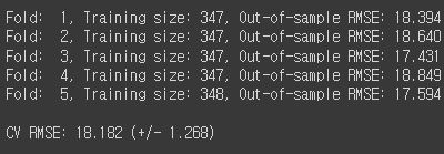
모델을 사용하는 방법은 위와 일치합니다. 중간에 모델만 바꿔주면 됩니다.
R-squared값이나 RMSE값이나 OLS모델 LinearRegression모델 둘다 선형회귀라 흡사하게 결과를 가져옵니다.
'개발새발 > 데이터분석' 카테고리의 다른 글
| [Python] 유방암 환자 분류 모델(Logistic Regression, KNN, LDA, SVM, Random Forest) (1) | 2024.01.27 |
|---|---|
| [Python] 공기질 데이터 분석(다양한 Regression) (0) | 2024.01.19 |
| [Python] youtube API를 활용한 동영상 및 채널 분석 (1) | 2024.01.15 |
| [Python] 당뇨환자 재입원 예측모델(one-hot encoding, optuna, shap) (2) | 2024.01.14 |
| [Python] 의류판매량예측(시계열,RandomForest) (2) | 2024.01.13 |