애완동물의 수요가 많아지는 만큼 유기되고 있는 애완동물의 숫자도 점점 더 커지고 있다.cm = confusion_matrix(y_test, y_preds) disp = ConfusionMatrixDisplay(confusion_matrix=cm, display_labels=['Not Adopted','Adopted']) disp.plot()
어떠한 특성을 가진 동물들이 입양이 잘 되는지 분석하고, 통제할 수 없는 변수와 통제 가능한 변수를 분류하여
입양이 되기 위해서는 어떤 프로필을 작성하는것이 좋을지 살펴보자.
1. 데이터 로드 및 체크
(1) 라이브러리 import
from datetime import datetime
from math import exp
from collections import defaultdict

# Manage data and statistics
import numpy as np
from numpy.random import default_rng, SeedSequence
import pandas as pd
from pandas.api.types import CategoricalDtype

from scipy import stats
from scipy.special import expit, logit
from scipy.stats.mstats import winsorize
from scipy.interpolate import interp1d, make_interp_spline, BSpline

# Plot data
import matplotlib as mpl
import matplotlib.pyplot as plt
from matplotlib.ticker import FormatStrFormatter
mpl.style.use('tableau-colorblind10')

import seaborn as sns
sns.set_style("white")
sns.set_context("notebook")

from IPython.display import HTML, Image, display, Markdown as md

# statsmodels
import patsy
from patsy import dmatrices
import statsmodels
import statsmodels.api as sm
import statsmodels.formula.api as smf
from statsmodels.iolib.summary2 import summary_col

# scikit-learn
from sklearn.utils import shuffle
from sklearn.preprocessing import StandardScaler, PolynomialFeatures

from sklearn.linear_model import LogisticRegression, LogisticRegressionCV
from sklearn.tree import DecisionTreeClassifier

from sklearn.model_selection import train_test_split, cross_val_score, LeaveOneOut, KFold
from sklearn.metrics import accuracy_score, precision_score, recall_score, f1_score, roc_auc_score, confusion_matrix, classification_report, ConfusionMatrixDisplay

# tensorflow
import tensorflow as tf

from tensorflow import keras
from tensorflow.keras import layers
(2) data check
petfinder.info()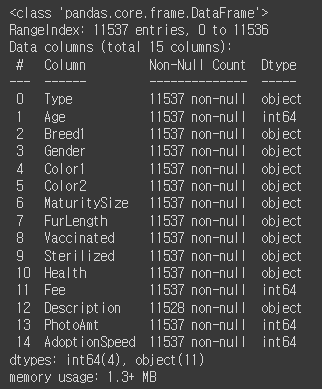
Description 열만 결측값이 존재하고 나머지는 결측값이 없다.
Age, Fee, PhotoAmt, AdoptionSeepd만 숫자형 데이터 이다.
petfinder.isna().sum()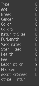
더블체크로 널값이 있는 열은 Description만 있는것을 확인
# 수치형 데이터를 가진 컬럼을 살펴보자.
petfinder.select_dtypes(include=np.number).columns.tolist()
>> ['Age', 'Fee', 'PhotoAmt', 'AdoptionSpeed']
petfinder[['Age']].hist(figsize=(10,5), bins=100)
250살 까지 사는 사람도 없는데 동물이 250살까지 나온다.
Age 열에서도 잘못입력된 행이 있을것이다.
petfinder.hist(figsize=(21,9))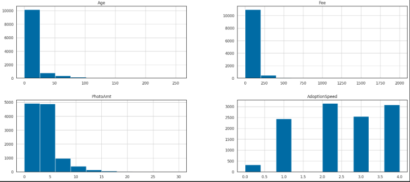
수치형 데이터들만 그래프로 확인해보았다.
입양이된 동물들이 대부분 4개월 이내로 입양이 된다.
petfinder.describe()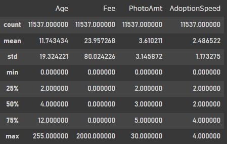
# In the original dataset, 'AdoptionSpeed' of 4 indicates a pet was not adopted.
petfinder['Adopted'] = np.where(petfinder['AdoptionSpeed']==4, 0, 1)

# Drop unused features.
petfinder = petfinder.drop(columns=['AdoptionSpeed', 'Description'])
petfinder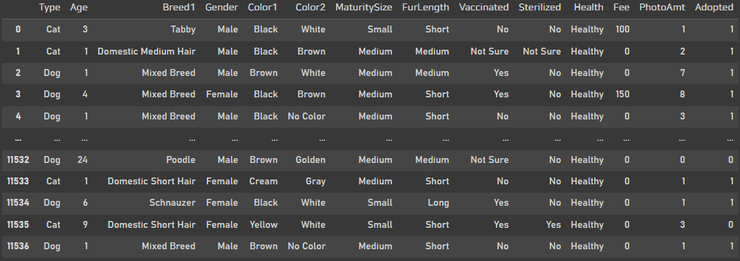
회귀모델을 사용하기위해서 입양된속도를 binary classification으로 바꾸어주었다.
3개월 이내까지는 1로 4개월은 0으로 바꿔주었다.
그리고 Description은 자연어라 처리하기 까다로워 drop진행했다.
features = petfinder.copy()
labels = features.pop('Adopted')

features.columns.tolist()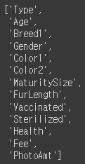
feature컬럼 지정
2. 데이터 전처리
features['Is_Cat'] = np.where(features['Type']=='Dog', 0., 1.)
features['Is_Female'] = np.where(features['Gender']=='Male', 0., 1.)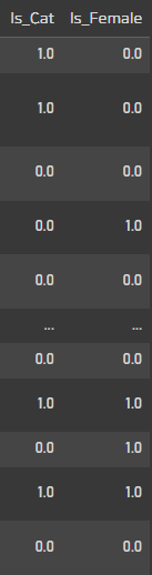
먼저 type에서 cat과 dog로 분리, 성별도 분리해주었다.
features['Vaccinated'].value_counts()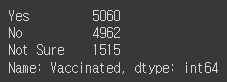
예방 접종이 되어있는 아이들을 확인하였는데, 2개가 아닌 3개로 나뉘어진다.
features = features.join(pd.get_dummies(features['Vaccinated'], prefix='Vaccinated'))
이런 경우 get_dummies를 이용해서 데이터에 추가해주었다.
features['Sterilized'].value_counts()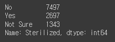
목욕이 된 친구들? 도 3개 카테고리
features['Health'].value_counts()
건강한지 안건강한지도 3개 카테고리
features = features.join(pd.get_dummies(features['Sterilized'], prefix='Sterilized'))
features = features.join(pd.get_dummies(features['Health'], prefix='Health'))
둘다 get_dummies로 추가해주었다.
features['MaturitySize'].unique()
동물들의 크기에도 3가지
털이 단모, 장모종인지에 따라서도 나뉘기 때문에 이것또한 같이 카테고리형으로 추가해주었다.
maturity_size_type = CategoricalDtype(categories=['Small', 'Medium', 'Large'], ordered=True)
features['MaturitySize'] = features['MaturitySize'].astype(maturity_size_type)
features = features.join(pd.get_dummies(features['MaturitySize'], prefix='MaturitySize'))

fur_length_type = CategoricalDtype(categories=['Short', 'Medium', 'Long'], ordered=True)
features['FurLength'] = features['FurLength'].astype(fur_length_type)
features = features.join(pd.get_dummies(features['FurLength'], prefix='FurLength'))

features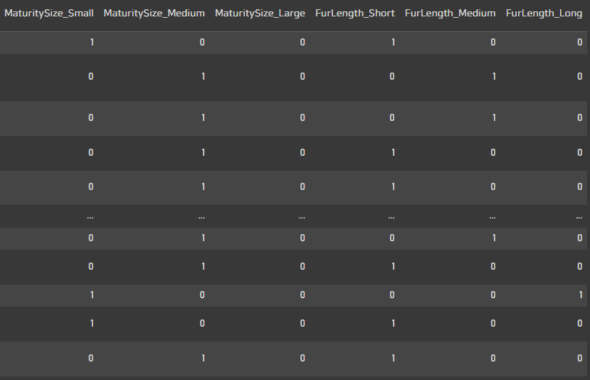
features['Color1'].unique()
features['Color2'].unique()
features = features.join(pd.get_dummies(features['Color1'], prefix='Color1'))
features = features.join(pd.get_dummies(features['Color2'], prefix='Color2'))
features
색상도 추가

ptile_labels = ['ptile1', 'ptile2', 'ptile3', 'ptile4', 'ptile5']
features = features.join(pd.get_dummies(pd.qcut(features['Age'], q=[0, .2, .4, .6, .8, 1], labels=ptile_labels), prefix='Age'))
features
나이의경우 하나하나 나눌수없어서 분위수를 이용해서 5개로 나뉘어 추가해주었다.
마지막 ptile5는 결측값으로 보고 drop시켜 사용할 예정이다.
features['Breed1'].value_counts()[:20]
keep_breeds = ['Mixed Breed', 'Domestic Short Hair', 'Domestic Medium Hair', 'Tabby',
               'Domestic Long Hair', 'Siamese', 'Shih Tzu', 'Labrador Retriever',
               'Persian', 'Poodle', 'Poodle', 'Terrier', 'Golden Retriever']

dd = defaultdict(lambda: 'Other')

for _, breed in enumerate(keep_breeds):
    dd[breed] = breed

features = features.join(pd.get_dummies(features['Breed1'].map(dd), prefix='Breed1'))
features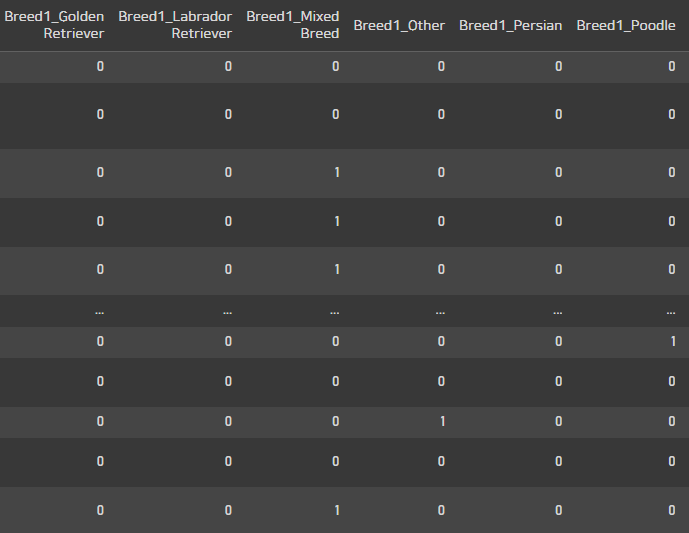
종의 경우는 너무 많은 데이터값이 있기 때문에
카운트가 100이 안넘는 종은 other값으로 통일
categorical_predictors = ['Type', 'Gender', 'Age', 'Color1', 'Color2', 'MaturitySize', 'FurLength', 'Vaccinated', 'Sterilized', 'Health', 'Breed1']카테고리형 범주로 바꾼 열 체크
predictors = [
  #'Type',
  #'Age',
  #'Breed1',
  #'Gender',
  #'Color1',
  #'Color2',
  #'MaturitySize',
  #'FurLength',
  #'Vaccinated',
  #'Sterilized',
  #'Health',
  #'Fee',
  'PhotoAmt',
  'Is_Cat',
  'Is_Female',
  #'Vaccinated_No',
  'Vaccinated_Not Sure',
  'Vaccinated_Yes',
  #'Sterilized_No',
  'Sterilized_Not Sure',
  'Sterilized_Yes',
  'Health_Healthy',
  'Health_Minor Injury',
  'Health_Serious Injury',
  'MaturitySize_Small',
  'MaturitySize_Medium',
  'MaturitySize_Large',
  'FurLength_Short',
  'FurLength_Medium',
  'FurLength_Long',
  #'Color1_Black',
  'Color1_Brown',
  'Color1_Cream',
  'Color1_Golden',
  'Color1_Gray',
  'Color1_White',
  'Color1_Yellow',
  'Color2_Brown',
  'Color2_Cream',
  'Color2_Golden',
  'Color2_Gray',
  #'Color2_No Color',
  'Color2_White',
  'Color2_Yellow',
  'Age_ptile1',
  'Age_ptile2',
  'Age_ptile3',
  'Age_ptile4',
  #'Age_ptile5',
  'Breed1_Domestic Long Hair',
  'Breed1_Domestic Medium Hair',
  'Breed1_Domestic Short Hair',
  'Breed1_Golden Retriever',
  'Breed1_Labrador Retriever',
  'Breed1_Mixed Breed',
  #'Breed1_Other',
  'Breed1_Persian',
  'Breed1_Poodle',
  'Breed1_Shih Tzu',
  'Breed1_Siamese',
  'Breed1_Tabby',
  'Breed1_Terrier'
]

features = features[predictors].copy()
# Standardized Mean Difference
features[predictors] = (features[predictors] - features[predictors].mean()) / features[predictors].std()
features
사용할 데이터를 평균차이에따른 오차를 수행해주었다.
값들이 다 표준화가 된것을 확인 할 수 있다.
features.describe().T.round(2)
행렬 전환.
features.hist(figsize=(21,24))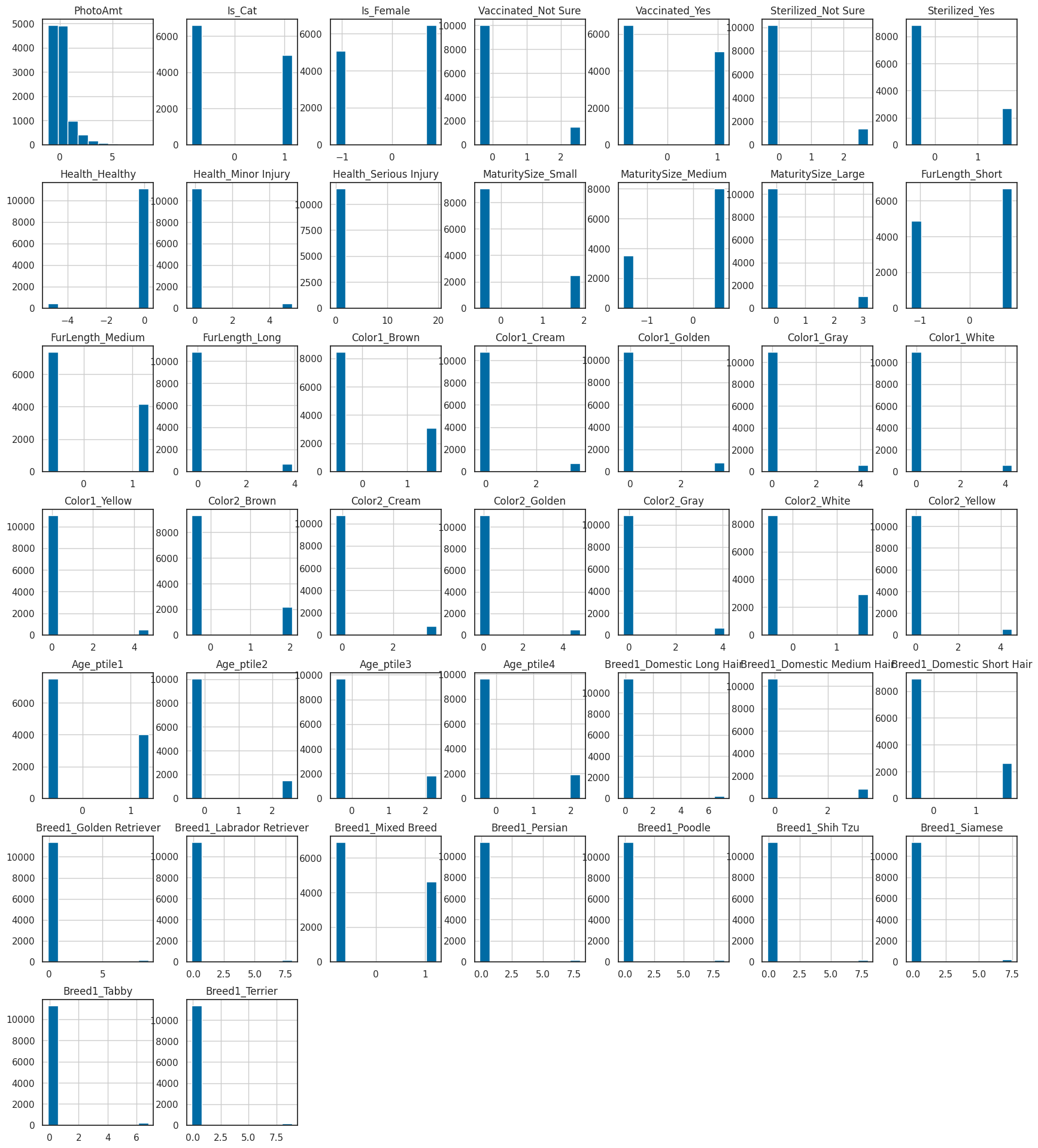
위에서 원래 사용하지 않으려던 데이터 말고
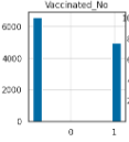
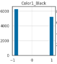
백신을 안맞은 동물들과 컬러가 블랙인 동물들은 비등비등하여 영향을 거의 미치지 않아 같이 제외해주었다.
X_train, X_test, y_train, y_test = train_test_split(features, labels, test_size=0.2, random_state=1234)데이터셋 분할 label로는 통제가능한 PhotoAmt 열을 사용했다.
g = sns.displot(X_train['PhotoAmt'], height=6, aspect=10/6)
g.set_axis_labels('Total uploaded photos for this pet (standardized)', '')
g.set_titles('')
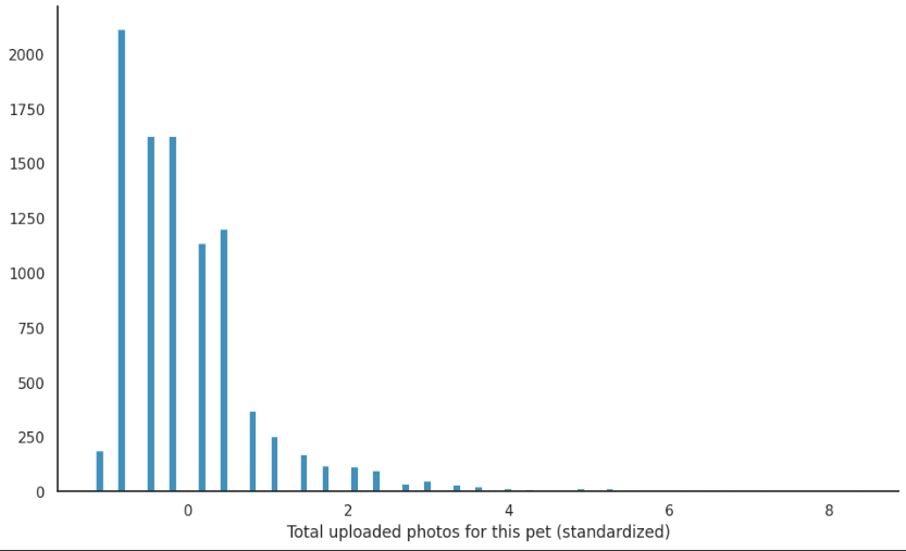
통제가능한 feature인 사진의 장수도 그래프로 한번 확인해주었다.
3. Modeling
(1) statsmodels
y = y_train.values

X = X_train['PhotoAmt'].values
X = sm.add_constant(X)

X.shape, y.shape
>> ((9229, 2), (9229,))
# Describe model
m1_sm = sm.Logit(y, X)

# Fit model
res_sm = m1_sm.fit()

# Summarize model
print(res_sm.summary())
coef가 1정도로 label값이 영향을 꽤나 미친다고 생각한다.
print("Parameters: ", [np.round(val, 2) for val in res_sm.params])
print("Standard errors: ", [np.round(val, 2) for val in res_sm.bse])
print("Predicted values: ", [np.round(val, 2) for val in res_sm.predict()[:10]])
세부 데이터도 확인
pd.concat([pd.Series(res_sm.predict(X)), pd.Series(expit(res_sm.fittedvalues))], axis=1).rename({0: 'Predicted', 1: 'Inverse Logit(Fitted)'}, axis=1)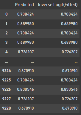
예측값과 Invese Logit 값을 확인해보면 똑같이 나온다.
res_sm_margeff = res_sm.get_margeff()
print(res_sm_margeff.summary())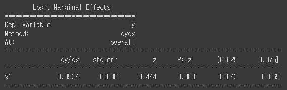
사진의 양이 많아질 수록 입양률도 증가할것같다.
fig, ax = plt.subplots(figsize=(10, 6))
sns.regplot(x='PhotoAmt', y='Adopted', data=X_train.join(pd.Series(labels, name='Adopted')),
            logistic=True, n_boot=500, x_jitter=.03, y_jitter=.03,
            scatter_kws={'alpha': 0.10}, # Set transparency to 10%
            ax=ax)
ax.set_ylabel('Pr(Adopted)', fontsize=14)
ax.set_xlabel('Total uploaded photos for this pet (standardized)', fontsize=14)
ax.set_title('Logistic Regression', fontsize=18);
그래프로 그려봤을때 사진의 양이 입양에 영향을 끼친다고 판단
def rand_jitter(arr):
    stdev = .01 * (max(arr) - min(arr))
    return arr + np.random.randn(len(arr)) * stdev # 표준화

x = np.linspace(X_train['PhotoAmt'].min(), X_train['PhotoAmt'].max(), 1000)
y = res_sm.predict(pd.DataFrame({'const': 1, 'PhotoAmt': x}))
f = interp1d(x, y, kind = "cubic")
xnew = np.linspace(X_train['PhotoAmt'].min(), X_train['PhotoAmt'].max(), 1000)
ynew = f(xnew)

fig, ax = plt.subplots(figsize=(10, 6))

ax.scatter(X_train['PhotoAmt'], rand_jitter(y_train), alpha=0.1, label='Data')
plt.plot(xnew, ynew, linestyle='-', color='black', label='Regression model')

ax.set_ylabel('Pr(Adopted)', fontsize=14)
ax.set_xlabel('Total uploaded photos for this pet (standardized)', fontsize=14)
ax.legend(fontsize=11)
ax.set_title('Logistic Regression', fontsize=18)

fig.tight_layout();
그래프의 밀도가 너무 높아 다시 그려주었다.
X_tests = X_test['PhotoAmt'].values
X_tests = sm.add_constant(X_tests)
y_pred_probs = res_sm.predict(exog=X_tests)
y_preds = list(map(round, y_pred_probs))
PhotoAmt값만 넣었을때의 결과를 확인해보자
cm = confusion_matrix(y_test, y_preds)
disp = ConfusionMatrixDisplay(confusion_matrix=cm, display_labels=['Not Adopted','Adopted'])
disp.plot()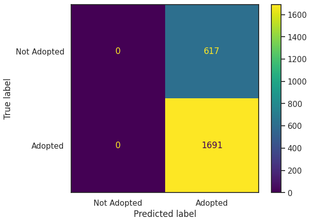
사진의 양만 많아진다고 입양이 다 되는 것은 아니다.
사진의양만 가지고 모델을 만들었더니 모두 입양된다고 나와버렸다.
print(classification_report(y_test, y_preds, target_names=['Not Adopted', 'Adopted']))
recall이 무려 1
모두 입양된다고 했는데 실제로 입양된건 73%정도 이다.
(2) scikit-learn
scikit-learn의 경우 statsmodel과 거의 흡사
y = y_train.values

X = X_train['PhotoAmt'].values
X = sm.add_constant(X)

X.shape, y.shape
>> ((9229, 2), (9229,))
coefs = [np.round(val, 4) for val in res_sk.coef_.flatten()]

ols_coefs = pd.DataFrame.from_dict( dict(zip(['Intercept', 'PhotoAmt'], coefs)), orient='index')
ols_coefs.columns = ['coef']

ols_coefslr = LogisticRegression(penalty='none', fit_intercept=False)

res_sk = lr.fit(X, y)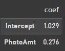
위에서 사용한 statsmodel과 같은 coef이 나왔다.
x = np.linspace(X_train['PhotoAmt'].min(), X_train['PhotoAmt'].max(), 1000)
y = res_sm.predict(pd.DataFrame({'const': 1, 'PhotoAmt': x}))
f = interp1d(x, y, kind = "cubic")
xnew = np.linspace(X_train['PhotoAmt'].min(), X_train['PhotoAmt'].max(), 1000)
ynew = f(xnew)

fig, ax = plt.subplots(figsize=(10, 6))

ax.scatter(X_train['PhotoAmt'], rand_jitter(y_train), alpha=0.1, label='Data')
plt.plot(xnew, ynew, linestyle='-', color='black', label='Regression model')

ax.set_ylabel('Pr(Adopted)', fontsize=14)
ax.set_xlabel('Total uploaded photos for this pet (standardized)', fontsize=14)
ax.legend(fontsize=11)
ax.set_title('Logistic Regression', fontsize=18)

fig.tight_layout();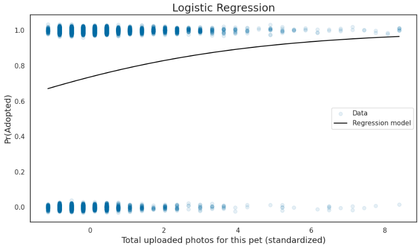
그래프도 확인해보면 일치
X_tests = X_test['PhotoAmt'].values
X_tests = sm.add_constant(X_tests)
y_pred_probs = res_sk.predict_proba(X_tests)
y_preds = res_sk.predict(X_tests)
confusion matrix도 일치
print(classification_report(y_test, y_preds, target_names=['Not Adopted', 'Adopted']))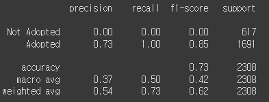
결과값도 확인해보면 일치한다.
(3) tensorflow
먼저, 데이터를 새로 읽어들여와서 깨끗한 데이터를 사용한다.
# In the original dataset, `'AdoptionSpeed'` of `4` indicates
# a pet was not adopted.
dataframe['target'] = np.where(dataframe['AdoptionSpeed']==4, 0, 1)

# Drop unused features.
dataframe = dataframe.drop(columns=['AdoptionSpeed', 'Description'])
위와 같이 입양속도를 보고 binary classcification으로 바꾸어 target값으로 지정
train, val, test = np.split(dataframe.sample(frac=1), [int(0.8*len(dataframe)), int(0.9*len(dataframe))])데이터셋 분할
def df_to_dataset(dataframe, shuffle=True, batch_size=32):
    df = dataframe.copy()
    labels = df.pop('target')
    df = {key: value[:,tf.newaxis] for key, value in dataframe.items()}
    ds = tf.data.Dataset.from_tensor_slices((dict(df), labels))
    if shuffle:
      ds = ds.shuffle(buffer_size=len(dataframe))
    ds = ds.batch(batch_size)
    ds = ds.prefetch(batch_size)
    return ds

def get_normalization_layer(name, dataset):
    normalizer = layers.Normalization(axis=None)
    feature_ds = dataset.map(lambda x, y: x[name])
    normalizer.adapt(feature_ds)

    return normalizer

def get_category_encoding_layer(name, dataset, dtype, max_tokens=None):
    if dtype == 'string':
        index = layers.StringLookup(max_tokens=max_tokens)
    else:
        index = layers.IntegerLookup(max_tokens=max_tokens)

    feature_ds = dataset.map(lambda x, y: x[name])
    index.adapt(feature_ds)
    encoder = layers.CategoryEncoding(num_tokens=index.vocabulary_size())

    return lambda feature: encoder(index(feature))
각각 df을 dataset으로 바꾸는 함수, normalization으로 변환함수, 카테고리로 인코딩하는 함수를 만들어주었다.
batch_size = 256
train_ds = df_to_dataset(train, batch_size=batch_size)
val_ds = df_to_dataset(val, shuffle=False, batch_size=batch_size)
test_ds = df_to_dataset(test, shuffle=False, batch_size=batch_size)
all_inputs = []
encoded_features = []
for header in ['PhotoAmt', 'Fee']: # 숫자형 컬럼 변환
numeric_col = tf.keras.Input(shape=(1,), name=header)
normalization_layer = get_normalization_layer(header, train_ds)
encoded_numeric_col = normalization_layer(numeric_col)
all_inputs.append(numeric_col)
encoded_features.append(encoded_numeric_col)feature로 사진의양 뿐만아니라 요금도 넣어보자.
age_col = tf.keras.Input(shape=(1,), name='Age', dtype='int64')

encoding_layer = get_category_encoding_layer(name='Age',
                                             dataset=train_ds,
                                             dtype='int64',
                                             max_tokens=5)
encoded_age_col = encoding_layer(age_col)
all_inputs.append(age_col)
encoded_features.append(encoded_age_col)
categorical_cols = ['Type', 'Color1', 'Color2', 'Gender', 'MaturitySize',
'FurLength', 'Vaccinated', 'Sterilized', 'Health', 'Breed1']
for header in categorical_cols:
categorical_col = tf.keras.Input(shape=(1,), name=header, dtype='string')
encoding_layer = get_category_encoding_layer(name=header,
dataset=train_ds,
dtype='string',
max_tokens=5)
encoded_categorical_col = encoding_layer(categorical_col)
all_inputs.append(categorical_col)
encoded_features.append(encoded_categorical_col)all_features = tf.keras.layers.concatenate(encoded_features)
x = tf.keras.layers.Dense(32, activation="relu")(all_features)
x = tf.keras.layers.Dropout(0.5)(x)
output = tf.keras.layers.Dense(1)(x)
model = tf.keras.Model(all_inputs, output)필요한 데이터들을 만든 함수를 이용해서 전처리해준다
model.compile(optimizer=tf.keras.optimizers.Adam(learning_rate=1e-3),
              loss=tf.keras.losses.BinaryCrossentropy(from_logits=True),
              metrics=['accuracy'])
모델 생성
# Use `rankdir='LR'` to make the graph horizontal.
tf.keras.utils.plot_model(model, show_shapes=True, rankdir="LR")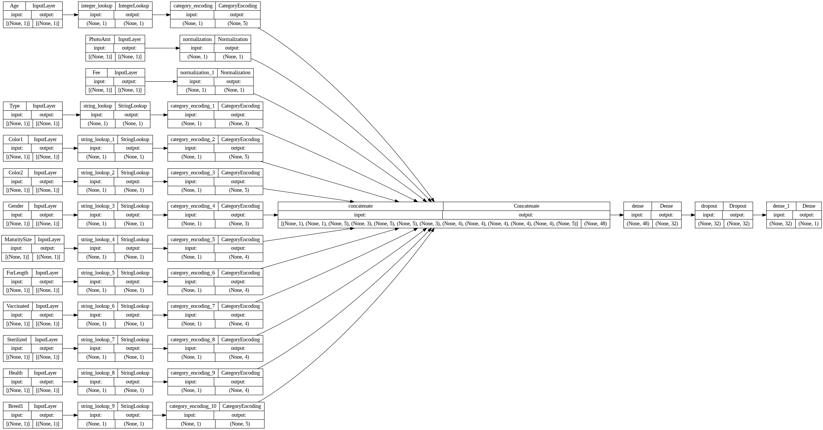
각각 나눠준 feature들이 병렬로 붙혀진것을 볼 수 있다.
baseline_history = model.fit(train_ds, epochs=10, validation_data=val_ds)
baseline_history
10번 epoch을 돌려 모델 학습해주었다.
loss, accuracy = model.evaluate(test_ds)
print("Accuracy", np.round(accuracy, 3))
정확도 위와 비슷하게 73%정도가 나왔다.
model.predict(test_ds).flatten()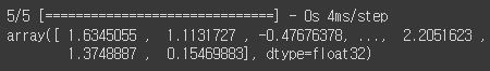
예측값 전처리해주고
cm = confusion_matrix((model.predict(test_ds) > 0.5).astype("int32").flatten(), test['target'].values)
disp = ConfusionMatrixDisplay(confusion_matrix=cm, display_labels=['Not Adopted','Adopted'])
disp.plot()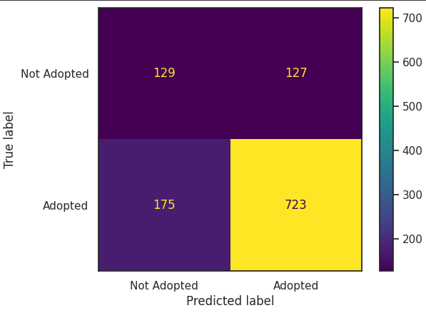
confusion matric를 찍어보았을때 Logistic Regression모델보다 좋게나왔다.
미입양 예측도 나오고 잘못예측된 부분도 확인 할 수 있다.
precision = precision_score((model.predict(test_ds) > 0.5).astype("int32").flatten(), test['target'].values)
recall    = recall_score((model.predict(test_ds) > 0.5).astype("int32").flatten(), test['target'].values)
print(classification_report((model.predict(test_ds) > 0.5).astype("int32").flatten(), test['target'].values, target_names=['Not Adopted','Adopted']))
전체적인 정확도는 비슷하나
전체를 입양으로 예측한것보다 훨씬 괜찮은 모델로 판단된다.
(4) 모델 비교
pd.DataFrame([[test_accuracy_sm, test_precision_sm, test_recall_sm],
              [test_accuracy_sk, test_precision_sk, test_recall_sk],
              [accuracy, precision, recall]],
             index=['statsmodels', 'scikit-learn', 'tensorflow'],
             columns=['Accuracy', 'Precision', 'Recall']).round(2)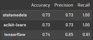
tensorflow를 사용했을때 전체 정확도가 가장 높고 예측도 높게 나왔다.
Deep learngin이 만능 알고리즘은 아니지만 시도해볼만한 모델이다.
4. 모델 저장 및 사용
모델이 큰경우 매번 학습해서 사용하는것이 아니라 저장해서 사용할 수 있는 방법
model.save('my_pet_classifier')
reloaded_model = tf.keras.models.load_model('my_pet_classifier')
sample = {
'Type': 'Dog',
'Age': 1,
'Breed1': 'Tabby',
'Gender': 'Female',
'Color1': 'Black',
'Color2': 'White',
'MaturitySize': 'Small',
'FurLength': 'Short',
'Vaccinated': 'No',
'Sterilized': 'No',
'Health': 'Healthy',
'Fee': 100,
'PhotoAmt': 10,
}
input_dict = {name: tf.convert_to_tensor([value]) for name, value in sample.items()}
predictions = reloaded_model.predict(input_dict)
prob = tf.nn.sigmoid(predictions[0])
print(
"This particular pet had a %.1f percent probability "
"of getting adopted." % (100 * prob)
)
여러개 넣어봤는데 확실히 사진의 양이 모델 정확도에 영향을 많이 주는것을 확인 할 수 있다.
'개발새발 > 데이터분석' 카테고리의 다른 글
| [Python] 신용카드 이상거래 탐지 모델(Undersampling, Oversampling) (2) | 2024.02.02 |
|---|---|
| [Python] E-commerce 행동 데이터 분석(RFM기반, Kmeans) (1) | 2024.01.31 |
| [Python] 유방암 환자 분류 모델(Logistic Regression, KNN, LDA, SVM, Random Forest) (1) | 2024.01.27 |
| [Python] 공기질 데이터 분석(다양한 Regression) (0) | 2024.01.19 |
| [Python] 자녀와 엄마의 IQ 상관관계 분석(OLS Regression, K-fold cross validation) (0) | 2024.01.18 |